In the first post in the taylor series, I introduced the taylor package for accessing data on Taylor Swift’s discography. In this post, we’ll dig into how one particular feature works under the hood: the custom color palettes.
First, credit where credit is due. This idea was 100% inspired by Josiah Parry’s work on the cpcinema package. That repository was a great starting point to build off of. Although I ended up re-building many of the functions to better suit the needs of taylor, this feature would not exist had I not seen this initial work. Second, the vctrs package has excellent documentation that makes building custom classes as straightforward as possible. Specifically, I spent a lot of time with the S3 vectors vignette. It’s a great resources for building your own classes. Without further ado, let’s get to it!
What do you mean ‘custom color palettes’?
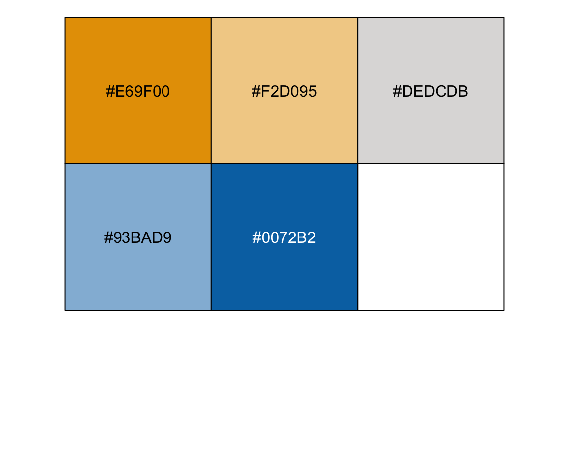
Let’s start with what we’re actually talking about. There are many ways to specify colors in R. For example, we can use any of the color names included in colors(), or we can specify our own hexadecimal values. And we can use scales::show_col() to see what these colors actually look like.
my_colors <- c("#E69F00", "#F2D095", "#DEDCDB", "#93BAD9", "#0072B2")
my_colors
#> [1] "#E69F00" "#F2D095" "#DEDCDB" "#93BAD9" "#0072B2"

scales::show_col(my_colors)
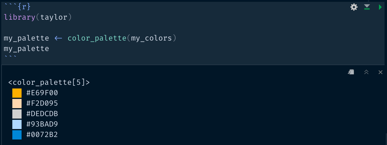
Using taylor, we can create a color palette with color_palette(). The color_palette() function returns the same vector of colors, but with a special print method to visualize the colors in the console.
library(taylor)

my_palette <- color_palette(my_colors)
my_palette
#> <color_palette[5]>
#>     #E69F00
#>     #F2D095
#>     #DEDCDB
#>     #93BAD9
#>     #0072B2
The blogdown package doesn’t currently support the type of syntax highlighting needed to display the full print method (there is an open issue on Github). But here’s what the output looks like rendered in my console:

Color palettes from taylor can be used just like a regular vector. However, we can also modify the palette as needed. By specifying the number of colors, n, we automatically interpolate between the colors originally specified, or pick a subset.
color_palette(my_palette, n = 15)
#> <color_palette[15]>
#>     #E69F00
#>     #E9AD2A
#>     #ECBB55
#>     #F0C97F
#>     #EFD19F
#>     #E9D5B3
#>     #E3D8C6
#>     #DEDCDB
#>     #C8D2DA
#>     #B3C8D9
#>     #9DBED9
#>     #7EAFD3
#>     #549BC8
#>     #2A86BD
#>     #0072B2

color_palette(my_palette, n = 3)
#> <color_palette[3]>
#>     #E69F00
#>     #DEDCDB
#>     #0072B2
In the rest of this post, we’ll look at how the vector class is defined.
Making a custom vctr
There are a few steps here, and we’ll follow the order in the S3 vectors vignette.
Step 1: Create an internal constructor function
We start by making a constructor function, new_color_palette(). This isn’t called directly by the user, but is used internally to create our new class. There are two arguments, pal, and n, which are used define the palette. In the body of the function, the first thing we do is use vctrs::vec_assert() to ensure that the values provided to the function arguments are in line with what we expect. Specifically, we expect pal to be a character vector, n to be a integer vector of length one.
We next figure out which colors to include in the palette. If no colors are specified (i.e., length(pal) = 0), we just keep the empty vector. If n is greater than the number of colors that were specified in pal, then we interpolate additional colors using grDevices::colorRampPalette(). Finally, if n is less than or equal to the number of colors specified in pal, we pull even spaced colors from pal.
The last step before creating the new vector is to figure out what to name each element of the palette. If pal is unnamed, we use the values as the names. If pal is named, we use the specified names.
We then create the new vector with vctrs::new_vctr(). The first argument, .data, is the vector we want to create a new class for. For our purposes, this is the vector of colors we just calculated. The next to arguments, n_colors and names get passed to the ... of vctrs::new_vctr() and will be attributes of the new vector class. Here, we store the number of colors in the palette and pass our names, nsm, to the names attribute. Finally, we give our class a name. Following the best practices the S3 vectors vignette, we prefix the class with "taylor_" to avoid namespace conflicts with other packages that might also have a color_palette class.
new_color_palette <- function(pal = character(), n = length(pal)) {
  vec_assert(pal, ptype = character())
  vec_assert(n, ptype = integer(), size = 1)

  out <- if (length(pal) == 0) {
    pal
  } else if (n > length(pal)) {
    grDevices::colorRampPalette(pal)(n)
  } else {
    index <- seq(1, length(pal), length.out = n)
    pal[as.integer(index)]
  }

  nms <- if (is.null(names(out))) out else names(out)

  new_vctr(.data = out,
           n_colors = n,
           names = nms,
           class = "taylor_color_palette")
}
Now that our constructor is done, we’re ready to make a user-friendly helper function.
Step 2: Create a user-facing helper
The purpose of the helper function is to be a little more forgiving with arguments and provide more informative error messages. The internal constructor requires a character vector input (because it uses vec_assert()). Here, we use vec_cast() to coerce the input to a character vector if possible. We then use two internal functions to make sure that the provided arguments have valid values. That is, although new_color_palette() uses vec_assert() to ensure that a character vector is supplied, not all character strings are valid colors. We can use some argument helper functions to check the values of the provided arguments. First, check_palette() verifies that the values supplied to pal are either (1) a valid hexadecimal code, or (2) a valid color from colors(). Second, check_pos_int() ensures that n is a positive integer greater than 0 (i.e., we can’t create a palette with a negative number of colors). The validated arguments are then passed to new_color_palette() to create the color palette.
Argument helper functions
check_palette <- function(x) {
  # look for R color specifications
  new_x <- x
  r_colors <- which(new_x %in% grDevices::colors())
  if (length(r_colors) > 0) {
    r_hex <- sapply(x[r_colors], function(.x) {
      r_rgb <- grDevices::col2rgb(.x)
      grDevices::rgb(red = r_rgb["red", 1], green = r_rgb["green", 1],
                     blue = r_rgb["blue", 1], maxColorValue = 255)
    })
    new_x[r_colors] <- r_hex
  }

  # make sure strings are valid hex codes
  valid_hex <- grepl("^#(?:[0-9a-fA-F]{6,8}){1}$", new_x)
  if (!all(valid_hex)) {
    rlang::abort(message = glue::glue("`pal` must be a valid hexadecimal",
                                      "value or from `colors()`.\n",
                                      "Problematic values: ",
                                      "{paste(x[!valid_hex], collapse = ', ')}"))
  }

  return(new_x)
}

check_pos_int <- function(x) {
  if (!is.numeric(x)) {
    rlang::abort(glue::glue("`n` must be numeric, not {typeof(x)}"))
  }

  if (length(x) != 1) {
    rlang::abort(glue::glue("`n` must be have length of 1, not {length(x)}"))
  }
  x <- as.integer(x)

  if (is.na(x)) {
    rlang::abort(glue::glue("`n` must be non-missing"))
  } else if (x < 0) {
    rlang::abort(glue::glue("`n` must be greater than 0"))
  } else {
    x
  }
}
color_palette <- function(pal = character(), n = length(pal)) {
# check palette and cast to character
pal <- vec_cast(pal, character())
pal <- check_palette(pal)
# check n
n <- check_pos_int(n)
new_color_palette(pal = pal, n = n)
}Step 3: Create custom printing
The final important step is to create the printing method that displays the color with the color name or hexadecimal code. This is accomplished with the obj_print_data.taylor_color_palette.default() function. This function defines the default method for printing data that has the taylor_color_palette class.
The key function here is crayon::make_style(). This function returns a function that will color strings. We use lapply() to create a list of functions, where each element is a function that will make the background (bg = TRUE) a color from pal. The final step is to use mapply() to map pal and the list of color functions, styles, to the cat() function.
Specifically, the printing is defined as cat("", .y(" "), .x, "\n"). We start with an empty string. We then add two spaces, which have a background color applied using the .y() function, which is the style function for the current color. Finally, we add the color name, .x, and put a line break at the end.
obj_print_data.taylor_color_palette.default <- function(pal, ...) {
  styles <- lapply(pal, crayon::make_style, bg = TRUE)
  invisible(
    mapply(
      function(.x, .y) {
        cat("", .y("  "), .x, "\n")
        return(invisible(.x))
      },
      vec_names(pal), styles,
      USE.NAMES = FALSE
    )
  )
}
Now when we print a color palette, we’ll see a rendering of the color, in addition to the colors’ names or hexadecimal codes!
Step 4: Miscellaneous infrastructure
There are many other helper functions that, if you are including your custom vector in a package, you should definitely include! However, I’m not including them here, as they’re not strictly necessary for this example. For example, in taylor, there are many functions for coercing and casting color palettes to characters and vice versa. For details, only these additional functions, I highly recommend the casting and coercion and implementing a vctrs S3 class in a package sections of the S3 vectors vignette.
Color palettes for taylor
In addition to the functionality to create color palettes, taylor also comes with several palettes built in. There is a color palette based on the cover art for each of Taylor Swift’s albums, which can be found in taylor::album_palettes. This is a list, where each element is a palette from one album. For example, we can view the palette for Lover with:
names(album_palettes)
#>  [1] "taylor_swift" "fearless"     "fearless_tv"  "speak_now"    "red"
#>  [6] "1989"         "reputation"   "lover"        "folklore"     "evermore"

album_palettes$lover
#> <color_palette[5]>
#>     #8C4F66
#>     #9C8083
#>     #847262
#>     #6098B6
#>     #EBBED3
Additionally, there is a palette that contains one representative color from each of the individual album palettes. This is useful if you are comparing albums directly against each other.
album_compare
#> <color_palette[10]>
#>     taylor_swift
#>     fearless
#>     fearless_tv
#>     speak_now
#>     red
#>     1989
#>     reputation
#>     lover
#>     folklore
#>     evermore
In the next post in this series, we’ll look at the ggplot2 scales that are included in taylor, and how they can be used to automatically apply these color palettes to graphics.
Acknowledgments
Featured photo by Robert Katzki on Unsplash.