
This time last year, I submitted a graphic to the Educational Measurement: Issues and Practice (EM:IP) cover showcase competition. In April at the annual National Council on Measurement in Education conference, it was announced that I was one of four winners that would be featured on the cover of EM:IP this year. Earlier this week, the issue with my graphic was released!
The graphic demonstrates how different levels of compensation in multidimensional item response theory models (MIRT). In this post, I’ll show how you can use R and ggplot2 to recreate the image.
Before demonstrating how to create the visualization, it will be useful to have brief explainer of item response theory. If you’d rather skip that, go ahead and go straight to the visualization.
A (somewhat) brief introduction to item response theory
Item response theory uses dichotomous or polytomous responses to a series of items in order to infer a respondent’s underlying latent ability. In traditional item response theory models, all of the items measure the same latent ability (e.g., all of the items measure “math ability”). In this type of model, the probability of respondent j answering item i correctly can be defined as
\[ P(X_{ij}=1\ |\ \theta_j) = c_i + (1-c_i)\frac{e^{a_i(\theta_j-b_i)}}{1 + e^{a_i(\theta_j-b_i)}} \]
This equation shows what is known as the 3 parameter logistic (3PL) item response theory model. In addition to θ, which represents the respondents ability, there are a, b, and c parameters for each item. This unidimensional model gives rise to an item characteristic curve for each item (for example, Figure 1).
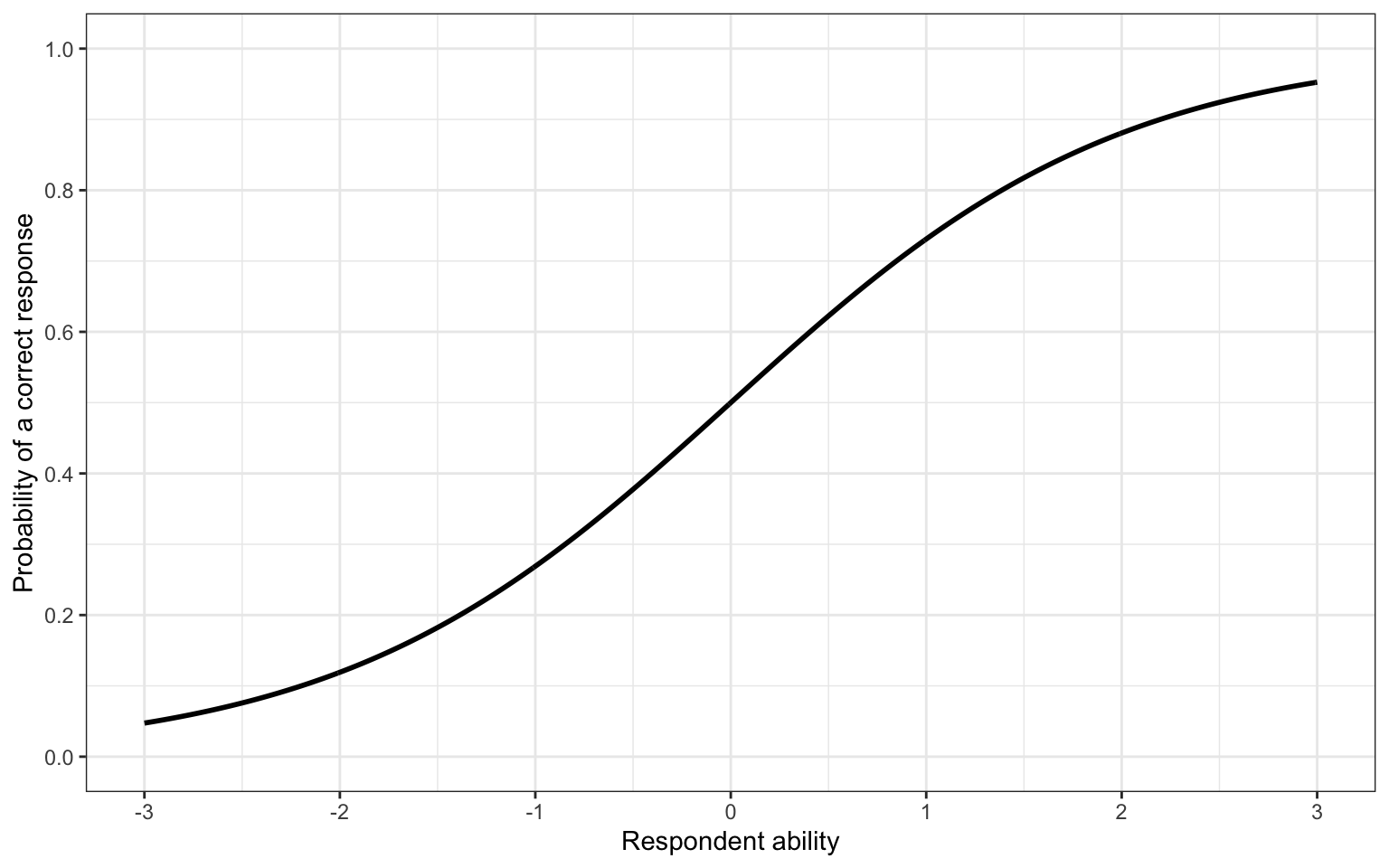
Figure 1: Example item characteristic curve
In Figure 1, we can see that as a respondent has higher ability, their probability of providing a correct response to the item increases, as we would expect. The a, b, and c parameters govern the shape of this line. The b parameter will shift the line left and right, meaning that a higher b parameter corresponds to a harder item. This is seen in Figure 2, where the probability of a correct response for the same level of ability is lower when the b parameter is larger.
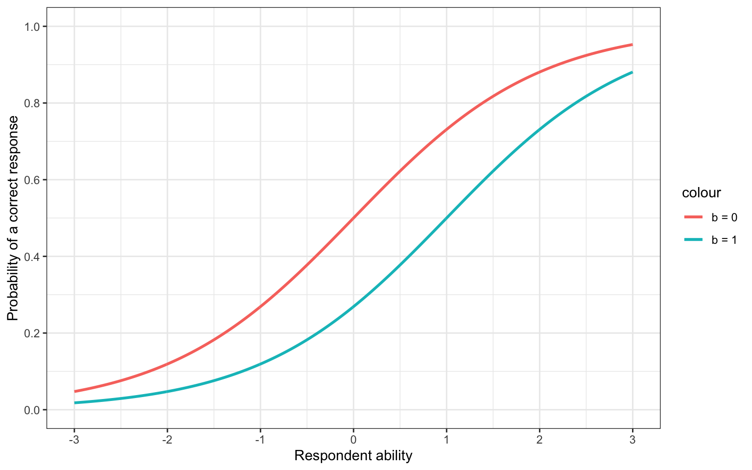
Figure 2: Shifting the b parameter
The a parameter influences the slope, or steepness, of the item characteristic curve. Larger a parameters result in a steeper line, meaning that the transition from a low probability of success to a high probability takes place over a smaller interval (Figure 3). This is also called the discrimination parameter, as items with a large a parameter are better able to discriminate respondets who have higher and lower ability.
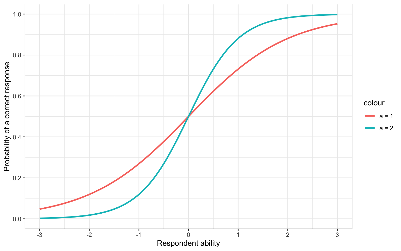
Figure 3: Shifting the a parameter
Finally, the c parameter defines the lower asymptote. This is also known as the guessing parameter. This is because if the c parameter is equal to 0.2, this means that no matter how low on ability a respondent is, they will never have less than a 20% chance of providing a correct response (Figure 4).
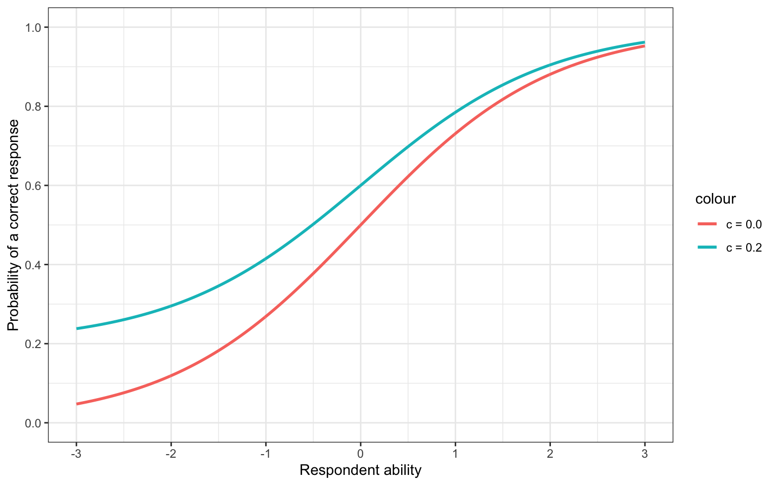
Figure 4: Shifting the c parameter
In Figure 2, Figure 3, and Figure 4, we only shifted one of the parameters, while the other two were held constant. In reality, all of the parameters would be estimated together. How many are estimated depends on the type of model. In addition to the 3PL model, there are also 2PL and 1PL variants. In the 2PL item response theory model, only the a and b parameters are estimated for each item, and the c parameter is fixed to 0. In the 1PL model, only the b is estimated for each item. In this version, the c parameter is again fixed to 0, and the a parameter is fixed to 1.
Multidimensional item response theory
So far we’ve looked at unidimensional item response theory models, where the probability of a correct response is determined by the ability on only one latent trait. In MIRT models, multiple latent traits contribute to a respondents probability of providing a correct response. In these models, rather than an item characteristic curve, there is an item characteristic plane that exists in multiple dimensions.
A key aspect of MIRT models is how the latent traits relate to each other. Specifically, we have decide whether a high level of ability on one trait is able to compensate for low levels of ability on another. Take for example a math word problem. We could reasonably argue that this item measures both math and reading ability. If we define a compensatory MIRT model, then a high level of either reading or math ability would allow for a high probability of providing a correct response. This type of model is defined as follows.
\[ P(X_{ij}=1\ |\ \boldsymbol{\theta}_j) = c_i + (1 - c_i)\frac{e^{\mathbf{a}_i^\prime(\boldsymbol{\theta}_j-d_i)}}{1 + e^{\mathbf{a}_i^\prime(\boldsymbol{\theta}_j-d_i)}} \]
This equation looks very similar to the 3PL model with a few important differences. First θ is now a vector of abilities for respondent j instead of just one ability. Additionally, instead of a b parameter, this model has a d parameter. In the unidimensional model, the d parameter would be equal to -ab. The MIRT model is just rearranged to be more similar to a linear predictor. Therefore, the interpretation of the a and d parameter is a less straightforward, which is why the b parameter is preferred in the unidimensional model. This compensatory model is also additive, meaning that the ability on each dimension adds to the overall probability of providing a correct response. So even if one dimension doesn’t add very much to the probability, a high ability on the second dimension can still provide a significant increase, thus compensating for the other dimension.
In contrast, a noncompensatory model is multiplicative. Practically this means that both abilities must be present in order for the respondent to have a high probability of success. This can be defined as
\[ P(X_{ij}=1\ |\ \boldsymbol{\theta}_j) = c_i+(1-c_i)\prod_{l=1}^L\frac{e^{a_{il}\theta_{jl}-d_{il}}}{1 + e^{a_{il}\theta_{jl}-d_{il}}} \]
Here, L refers to the number of dimensions measured by the item (two in our math word problem example). Because the probability from each dimension is multiplied by the others, a low probability on any dimension will result in a low probability overall. Thus, a respondent needs to have a high ability on all dimensions, as other dimensions cannot compensate for the lack of another.
Finally, there is a middle ground between the fully compensatory and noncompensatory models. Instead of defining the abilities as either compensatory or noncompensatory, the partially compensatory model actually estimates the amount of compensation that is present.
\[ P(X_{ij} = 1\ |\ \boldsymbol{\theta_j})=c_i + (1-c_i)\frac{e^{a_{1i}\theta_{1j} + a_{2i}\theta_{2j} + a_{3i}\theta_{1j}\theta_{2j}-d_i}}{1 + e^{a_{1i}\theta_{1j} + a_{2i}\theta_{2j} + a_{3i}\theta_{1j}\theta_{2j}-d_i}} \]
With this model, there is an increase in the probability for each dimension, but also an estimated interaction term that dictates how much compensation is present.
Visualizing compensation in MIRT models
For me, it’s much easier to understand compensation in MIRT models through visualization than equations. The first step to creating this visualization is defining functions to calculate the probability of a correct response under each MIRT model given a resondent’s ability (x and y), and the model parameters.
logit <- function(x) {
  exp(x) / (1 + exp(x))
}
comp <- function(x, y, a1 = 1, a2 = 1, d = 0, c = 0) {
  lin_comb <- (a1 * x) + (a2 * y)
  c + (1 - c) * logit(lin_comb - d)
}
noncomp <- function(x, y, a1 = 1, a2 = 1, d1 = 0, d2 = 0, c = 0) {
  c + (1 - c) * prod(logit((a1 * x) - d1), logit((a2 * y) - d2))
}
partcomp <- function(x, y, a1 = 1, a2 = 1, a3 = 0.3, d = 0, c = 0) {
  c + (1 - c) * logit((a1 * x) + (a2 * y) + (a3 * x * y) - d)
}
Next, we simulate data from each of the MIRT models, using the 1PL, 2PL, and 3PL variants. For all models, the d parameter is fixed to zero, and the interaction term is fixed to 0.3 in the partial compensatory model for the 1PL, 2PL and 3PL variants. In the 2PL, we use an a parameter of 0.8 for the first dimension and 1.8 for the second. Finally, for the 3PL model, we use the same a parameters as in the 2PL model, and set the c parameter to 0.2.
We set the range of θ on both dimensions to range from -3 to 3. The crossing function from the tidyr package creates a data frame of all combinations of the two abilities. Finally, we use the map2_dbl function from the purrr package calculate the probability of a correct response for a respondent with each combination of abilities, and the specified item parameters.
theta_1 <- seq(-3, 3, 0.01)
theta_2 <- seq(-3, 3, 0.01)

pl1 <- crossing(theta_1, theta_2) %>%
  mutate(
    Model = "1PL",
    Compensatory = map2_dbl(.x = theta_1, .y = theta_2, .f = comp),
    Noncompensatory = map2_dbl(.x = theta_1, .y = theta_2, .f = noncomp),
    Partial = map2_dbl(.x = theta_1, .y = theta_2, .f = partcomp, a3 = 0.3)
  )

pl2 <- crossing(theta_1, theta_2) %>%
  mutate(
    Model = "2PL",
    Compensatory = map2_dbl(.x = theta_1, .y = theta_2, .f = comp,
      a1 = 0.8, a2 = 1.8),
    Noncompensatory = map2_dbl(.x = theta_1, .y = theta_2, .f = noncomp,
      a1 = 0.8, a2 = 1.8),
    Partial = map2_dbl(.x = theta_1, .y = theta_2, .f = partcomp,
      a1 = 0.8, a2 = 1.8, a3 = 0.3)
  )

pl3 <- crossing(theta_1, theta_2) %>%
  mutate(
    Model = "3PL",
    Compensatory = map2_dbl(.x = theta_1, .y = theta_2, .f = comp,
      a1 = 0.8, a2 = 1.8, c = 0.2),
    Noncompensatory = map2_dbl(.x = theta_1, .y = theta_2, .f = noncomp,
      a1 = 0.8, a2 = 1.8, c = 0.2),
    Partial = map2_dbl(.x = theta_1, .y = theta_2, .f = partcomp,
      a1 = 0.8, a2 = 1.8, a3 = 0.3, c = 0.2)
  )
Once the probabilities for each MIRT model under each of the 1PL, 2PL, and 3PL variants have been calculate, we can combine them, and make the plot!
bind_rows(pl1, pl2, pl3) %>%
  gather(Method, Probability, Compensatory:Partial) %>%
  mutate(Method = factor(Method, levels = c("Compensatory", "Partial",
    "Noncompensatory"), labels = c("Compensatory", "Partially Compensatory",
      "Noncompensatory"))) %>%
  ggplot(mapping = aes(x = theta_1, y = theta_2)) +
  facet_grid(Model ~ Method) +
  geom_raster(aes(fill = Probability), interpolate = TRUE) +
  geom_contour(aes(z = Probability), color = "black", binwidth = 0.1) +
  scale_x_continuous(breaks = seq(-10, 10, 1)) +
  scale_y_continuous(breaks = seq(-10, 10, 1)) +
  scale_fill_distiller(name = "Probability of Correct Response",
    palette = "Spectral", direction = -1, limits = c(0, 1),
    breaks = seq(0, 1, 0.1)) +
  labs(x = expression(paste(theta[1])), y = expression(paste(theta[2]))) +
  theme_minimal() +
  theme(
    aspect.ratio = 1,
    legend.position = "bottom",
    legend.title = element_text(vjust = 0.5, size = 14),
    legend.text = element_text(size = 12),
    axis.text = element_text(size = 12),
    axis.title = element_text(size = 14),
    strip.text = element_text(face = "bold", size = 14),
    legend.key.width = unit(1, "inches")
  ) +
  guides(fill = guide_colorbar(title.position = "top", title.hjust = 0.5))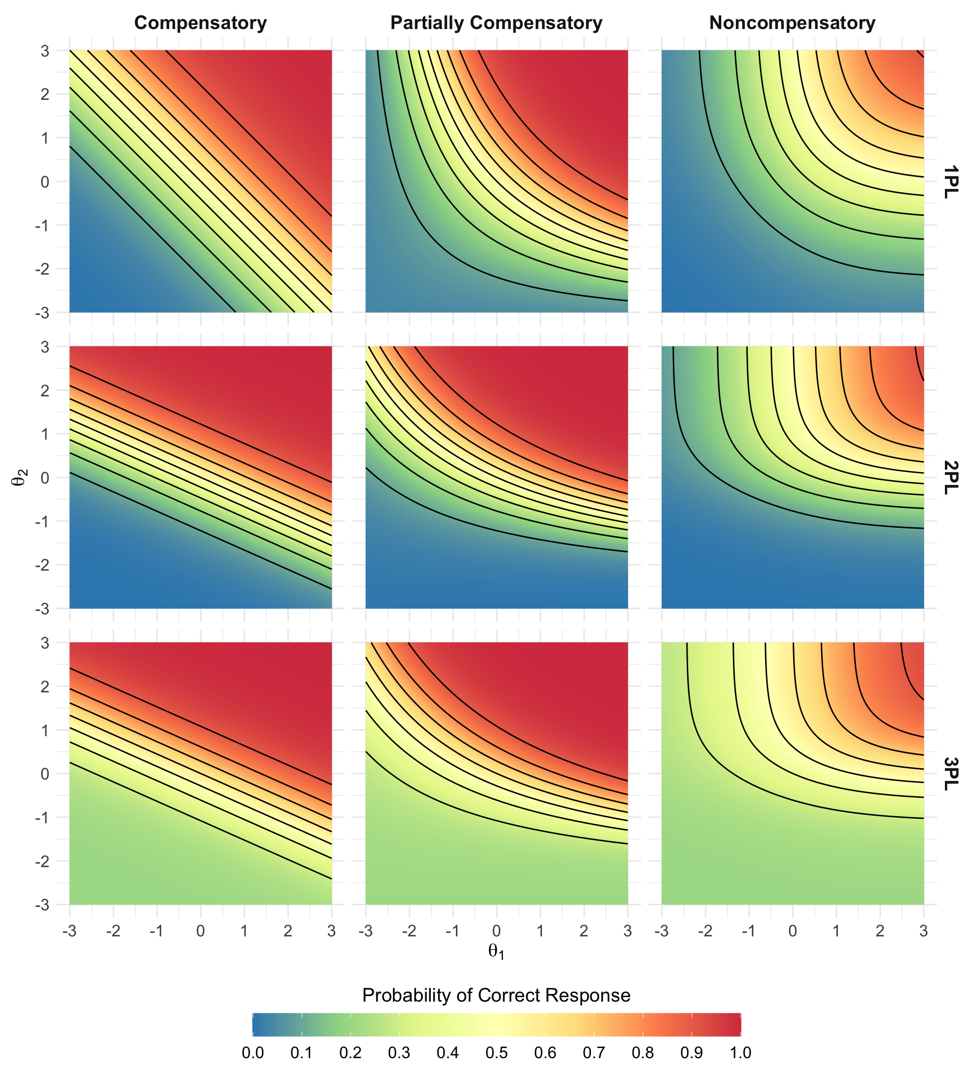
Figure 5: Visualizing different levels of compensation in multidimensional item response theory models
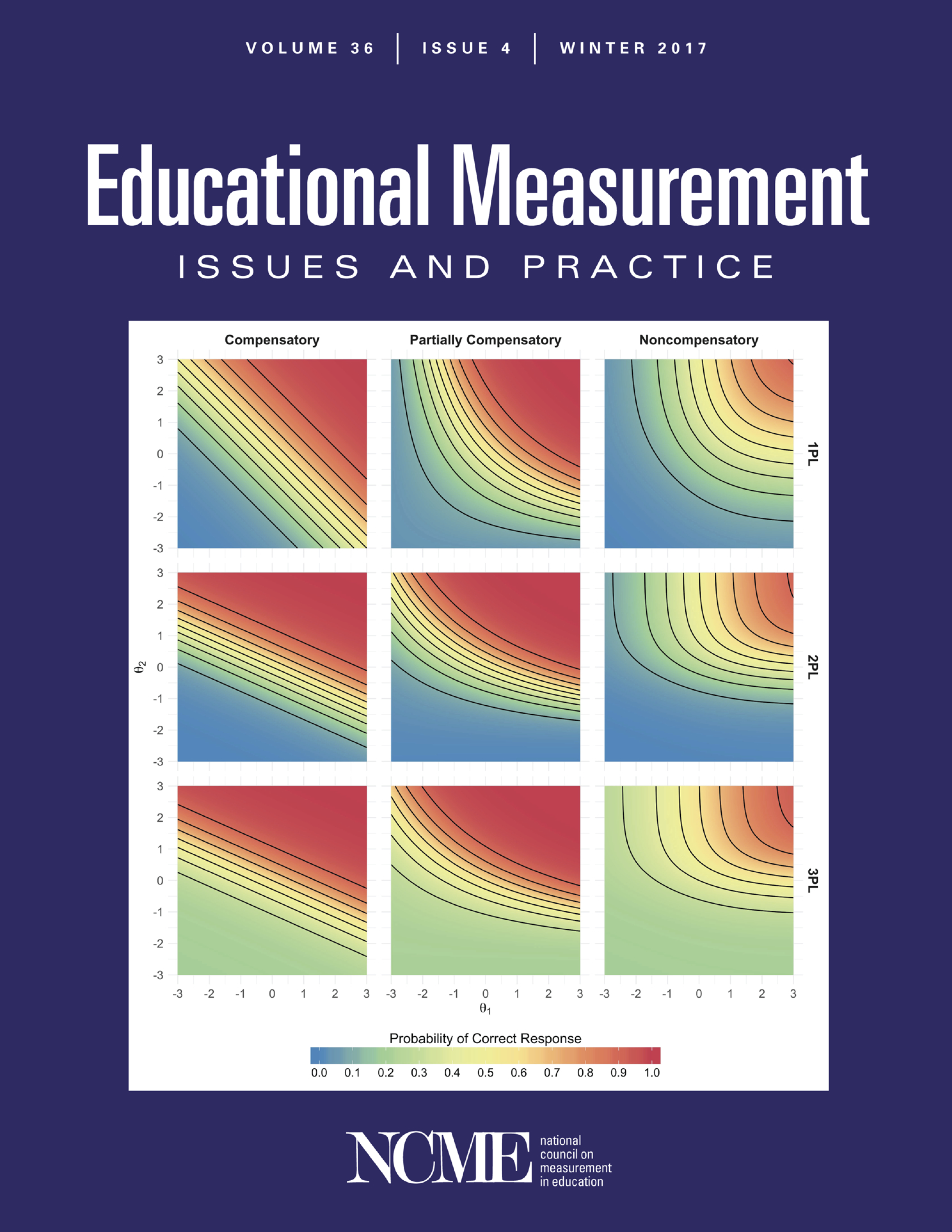
Figure 5 is the graphic that is printed on the cover. It is described in the journal as follows:
This graphic shows the probability of providing a correct response to an item in a multidimensional item response theory (MIRT) model. The colors represent the probability of a correct response, and the contours represent chunk of 10% probability (i.e., the space between the leftmost and second contours represents ability pairs with a 10-20% probability of answering correctly).
In this example, I use a 2-dimensional model to illustrate how the probabilities change depending on the parameterization of the model. In the compensatory model, one dimension is able to compensate for the other, whereas in the noncompensatory model, an individual needs high ability on both dimensions to have a high probability of success. The partially compensatory model is parameterized with an interaction term that allows one dimension to partially compensate for the other.
In the 1PL versions of these models, the b-parameters are set to 0, and the discriminations are fixed at 1, making this equivalent to the multidimensional Rasch model. In the 2PL versions, the discrimination is set to 0.8 for the first dimension and 1.8 for the second dimension. Accordingly, we can see the item get easier for individuals with low ability on dimension 1 and harder for individuals with low ability on dimension 2. Finally, in the 3PL versions, the c-parameter is set to 0.2, and we can see the probability level off at 0.2, rather than reaching all the way down to 0 for individuals with low ability on both dimensions. In all of the partially compensatory models, the discrimination for the interaction term is 0.3.
These plots show the 1PL, 2PL, and 3PL MIRT models are affected by how compensatory the model is parameterized to be. Additionally, creating 2-dimensional representations of the 3-dimensional curves makes it easier to identify differences in between the partially compensatory and noncompensatory models that tend to look very similar when rendered in 3 dimensions.
Acknowledgments
Featured photo by Jess Bailey on Unsplash.