In the first post in the taylor series, I introduced the taylor package for accessing data on Taylor Swift’s discography. We then began exploring some of the internals of the package by examining how taylor uses vctrs to create a custom color palette class. In this post, we’ll extend that work to see how the color palettes can be wrapped into color and fill scales for ggplot2.
ggplot2 scales
There are several ggplot2 scales included in taylor based on the album-inspired color palettes. These are:
scale_fill_taylor_c()for continuous scales,scale_fill_taylor_d()for discrete scales, andscale_fill_tayloy_b()for binned scales.
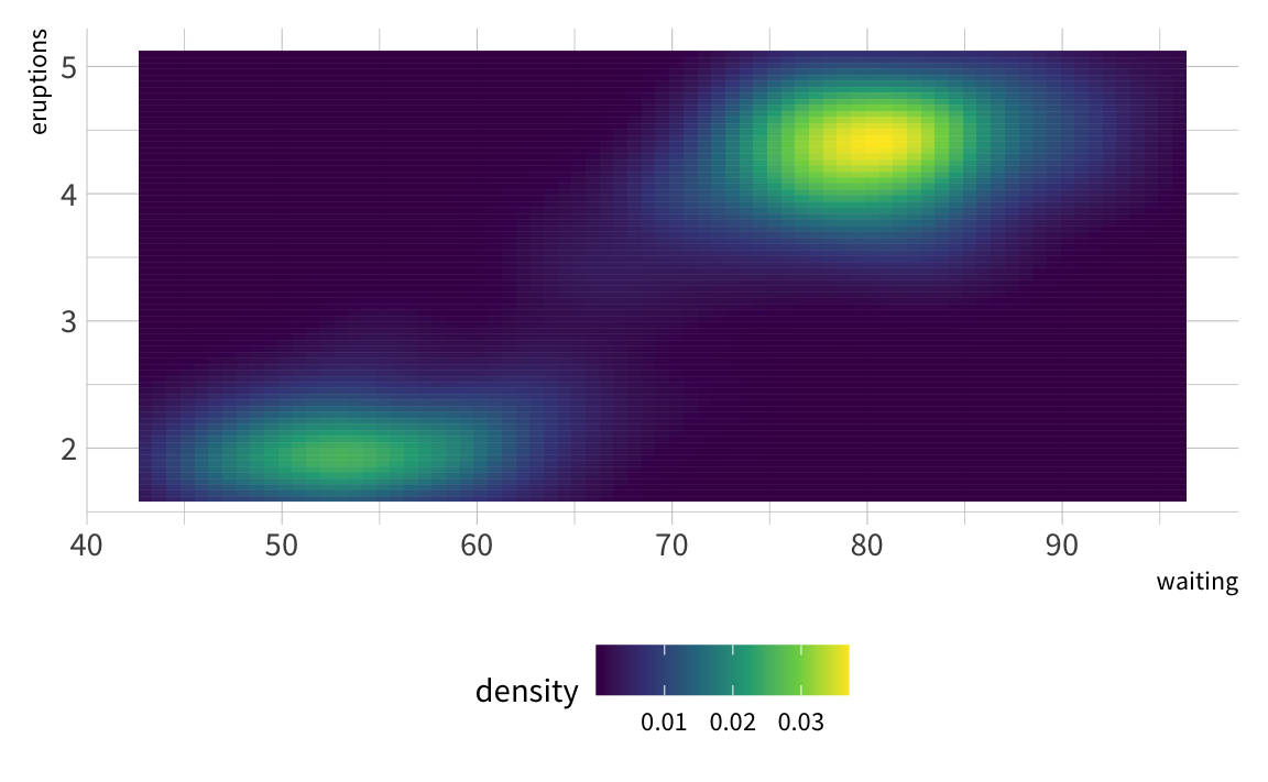
In addition, there are scale_color_taylor_*() variants that map to the color aesthetic rather than the fill aesthetic. These scale can be applied just like any other ggplot2 scale. For example, here is the default ggplot2 color palette.
p <- ggplot(faithfuld, aes(x = waiting, y = eruptions, fill = density)) +
  geom_tile()

p
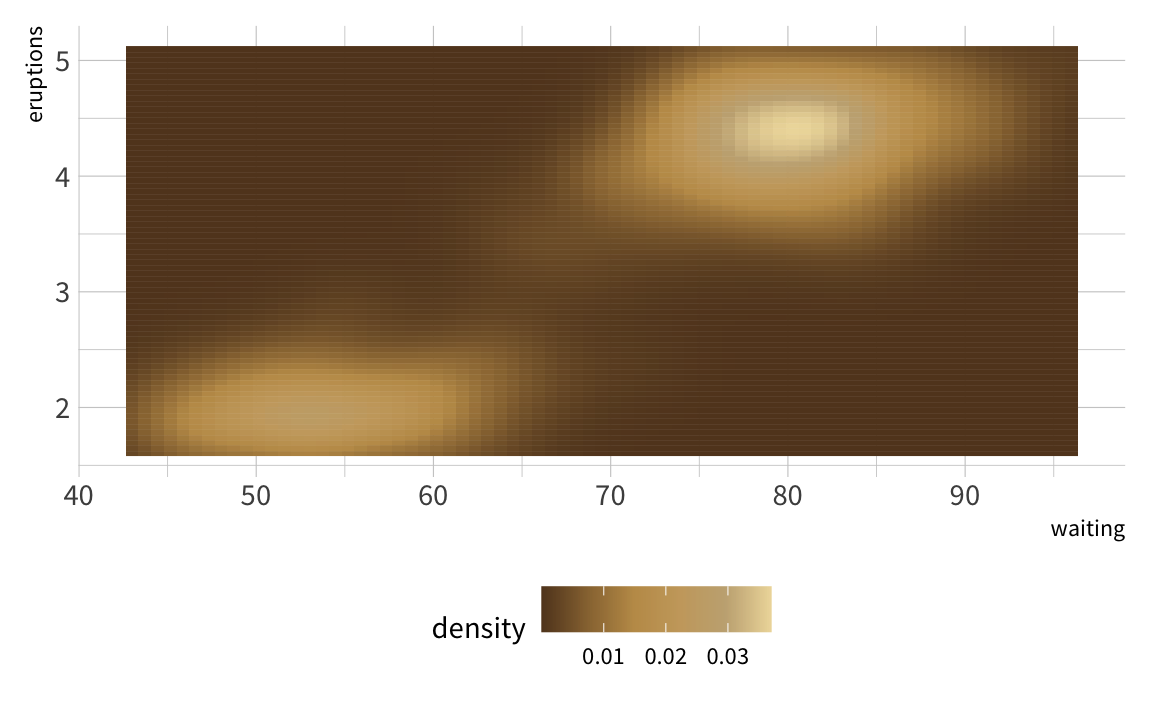
By default, the viridis palette is used for continuous scales. We can update to a Taylor Swift themed palette using scale_fill_taylor_c().
library(taylor)

p +
  scale_fill_taylor_c(album = "Fearless (Taylor's Version)")
In this post, we’ll dig into how the scale_fill_taylor_*() functions are built.
Building ggplot2 scales
To create the ggplot2 scales in taylor, I used the scale_fill_viridis_*() functions from ggplot2 as a template. Using these as a template, there were three major functions, or sets of functions, to write. We’ll walk through each in order.
Function 1: Generating colors for the scale
The main function that does most of the work for the ggplot2 scales in taylor is an internal function, taylor_col(). Here’s the function code, and then we’ll parse what is happening.
taylor_col <- function(n, alpha = 1, begin = 0, end = 1, direction = 1,
                       album = "Lover") {

  if (direction == -1) {
    tmp <- begin
    begin <- end
    end <- tmp
  }

  lookup_pal <- tolower(album)
  lookup_pal <- gsub("\\ ", "_", lookup_pal)
  lookup_pal <- gsub("\\(taylor's_version\\)", "tv", lookup_pal)

  option <- switch(EXPR = lookup_pal,
                   taylor_swift = taylor::album_palettes[["taylor_swift"]],
                   fearless     = taylor::album_palettes[["fearless"]],
                   fearless_tv  = taylor::album_palettes[["fearless_tv"]],
                   speak_now    = taylor::album_palettes[["speak_now"]],
                   red          = taylor::album_palettes[["red"]],
                   `1989`       = taylor::album_palettes[["1989"]],
                   reputation   = taylor::album_palettes[["reputation"]],
                   lover        = taylor::album_palettes[["lover"]],
                   folklore     = taylor::album_palettes[["folklore"]],
                   evermore     = taylor::album_palettes[["evermore"]], {
                     rlang::warn(paste0("Album '", album, "' does not exist. ",
                                        "Defaulting to 'Lover'."))
                     taylor::album_palettes[["lover"]]
                   })

  fn_cols <- grDevices::colorRamp(option, space = "Lab",
                                  interpolate = "spline")
  cols <- fn_cols(seq(begin, end, length.out = n)) / 255
  grDevices::rgb(cols[, 1], cols[, 2], cols[, 3], alpha = alpha)
}
This function takes six arguments: n is the number of colors, alpha defines the transparency, begin and end specify the range of the palette to use, direction specifies which end of the palette should be the starting end, and finally album is the album palette that should be used.
The first bit of code flips the begin and end values if we choose to reverse the direction. For example, if we want to go from 1 to 0 instead of 0 to 1.
if (direction == -1) {
    tmp <- begin
    begin <- end
    end <- tmp
}
Next, we parse the the album name to identify the palette. The intention is for users to be able to specify an album using the normal album name (e.g., Speak Now). However, the album_palettes object uses names that are more friendly to R.
names(album_palettes)
#>  [1] "taylor_swift" "fearless"     "fearless_tv"  "speak_now"    "red"
#>  [6] "1989"         "reputation"   "lover"        "folklore"     "evermore"
To convert the true album name to the version that is used in album_palettes, we convert all the letters to lower case, replace spaces with underscores, and finally replace taylor's_version with tv.
lookup_pal <- tolower(album)
lookup_pal <- gsub("\\ ", "_", lookup_pal)
lookup_pal <- gsub("\\(taylor's_version\\)", "tv", lookup_pal)
This converted lookup_pal can then be used to select the chosen color palette using switch(). The converted album name is used as the EXPR, and for each the corresponding element of album_palettes is selected. The last argument of switch is a warning. If the converted lookup_pal doesn’t correspond to any element of album_palettes, the Lover palette is used.
option <- switch(EXPR = lookup_pal,
                 taylor_swift = taylor::album_palettes[["taylor_swift"]],
                 fearless     = taylor::album_palettes[["fearless"]],
                 fearless_tv  = taylor::album_palettes[["fearless_tv"]],
                 speak_now    = taylor::album_palettes[["speak_now"]],
                 red          = taylor::album_palettes[["red"]],
                 `1989`       = taylor::album_palettes[["1989"]],
                 reputation   = taylor::album_palettes[["reputation"]],
                 lover        = taylor::album_palettes[["lover"]],
                 folklore     = taylor::album_palettes[["folklore"]],
                 evermore     = taylor::album_palettes[["evermore"]], {
                   rlang::warn(paste0("Album '", album, "' does not exist. ",
                                      "Defaulting to 'Lover'."))
                   taylor::album_palettes[["lover"]]
                 })
Finally, we’re ready to create the colors for the scale. First, we use grDevices::colorRamp() to create a new function, fn_cols that can interpolate values between the colors specified in color palette. Then, we use that function to generate a matrix of colors in RGB form. The matrix will have three columns (one each for red, green, and blue), and rows equal to n. The last step is to call grDevices::rgb(), which takes the red, green, and blue columns from cols and the alpha argument, and returns hexadecimal code for each of the final colors.
fn_cols <- grDevices::colorRamp(option, space = "Lab",
                                interpolate = "spline")
cols <- fn_cols(seq(begin, end, length.out = n)) / 255
grDevices::rgb(cols[, 1], cols[, 2], cols[, 3], alpha = alpha)
Now that we have a function that generates the colors from an album palette, we’re ready to start wrapping functions into ggplot2 scales.
Function 2:
The next function to make is also an internal function. This function, taylor_pal() is what’s known as a function factory. That is, taylor_pal() is a function that returns another function.
taylor_pal <- function(alpha = 1, begin = 0, end = 1, direction = 1,
                       album = "Lover") {
  function(n) {
    taylor_col(n, alpha, begin, end, direction, album)
  }
}
Specifically, it returns a function that takes one argument, n, and then passes a bunch of arguments onto the first function we made, taylor_col(). There’s not much else exciting happening here, other than this sets us up for our final function…
Function 3: ggplot2 scales
The step is to create the ggplot2 scales. There are three color scales for continuous, discrete, and binned data. All of these functions will wrap existing ggplot2 functionality.
We’ll start with the continuous scale, scale_colour_taylor_c(). The argument are the same as those for ggplot2::scale_colour_viridis_c(), with the additional of an extra album argument. We use ggplot2::continuous_scale() to construct the continuous scale. First we specify the aestheics (i.e., colour), and then provide a scale name. Next, is the palette. This is created by passing our previously created taylor_pal() function to scales::gradient_n_pal(). Finally, we specify the color for missing values and the type of guide to use as a legend. And that’s it!
scale_colour_taylor_c <- function(..., alpha = 1, begin = 0, end = 1,
                                  direction = 1, album = "Lover", values = NULL,
                                  space = "Lab", na.value = "grey50",
                                  guide = "colourbar", aesthetics = "colour") {
  ggplot2::continuous_scale(
    aesthetics,
    "taylor_c",
    scales::gradient_n_pal(
      taylor_pal(alpha, begin, end, direction, album)(6),
      values,
      space
    ),
    na.value = na.value,
    guide = guide,
    ...
  )
}
We can follow a similar process for discrete and binned scales. The main difference is that scale_colour_taylor_d() wraps ggplot2::discrete_scale() and scale_colour_taylor_b() wraps ggplot2::binned_scale(). Similar functions can also be created for mapping color to the fill by changing the aesthetic that is passed to the ggplot2 function.
scale_colour_taylor_d <- function(..., alpha = 1, begin = 0, end = 1,
                                  direction = 1, album = "Lover",
                                  aesthetics = "colour") {
  ggplot2::discrete_scale(
    aesthetics,
    "taylor_d",
    taylor_pal(alpha, begin, end, direction, album),
    ...
  )
}

scale_colour_taylor_b <- function(..., alpha = 1, begin = 0, end = 1,
                                  direction = 1, album = "Lover", values = NULL,
                                  space = "Lab", na.value = "grey50",
                                  guide = "coloursteps",
                                  aesthetics = "colour") {
  ggplot2::binned_scale(
    aesthetics,
    "taylor_b",
    scales::gradient_n_pal(
      taylor_pal(alpha, begin, end, direction, album)(6),
      values,
      space
    ),
    na.value = na.value,
    guide = guide,
    ...
  )
}
That’s all there is two it! I will note that this isn’t strictly necessary. We could have used the album_palettes with ggplot2 by using ggplot2::scale_color_gradientn(). But where’s the fun in that?!
This is the last post for now digging into the internals of taylor. However, you can expect a new release post soon, as Red (Taylor’s Version) is being released in just a few hours!

Acknowledgments
Featured photo by Pawel Czerwinski on Unsplash.